Quick Start
It's easier than you think
Installation (from source)
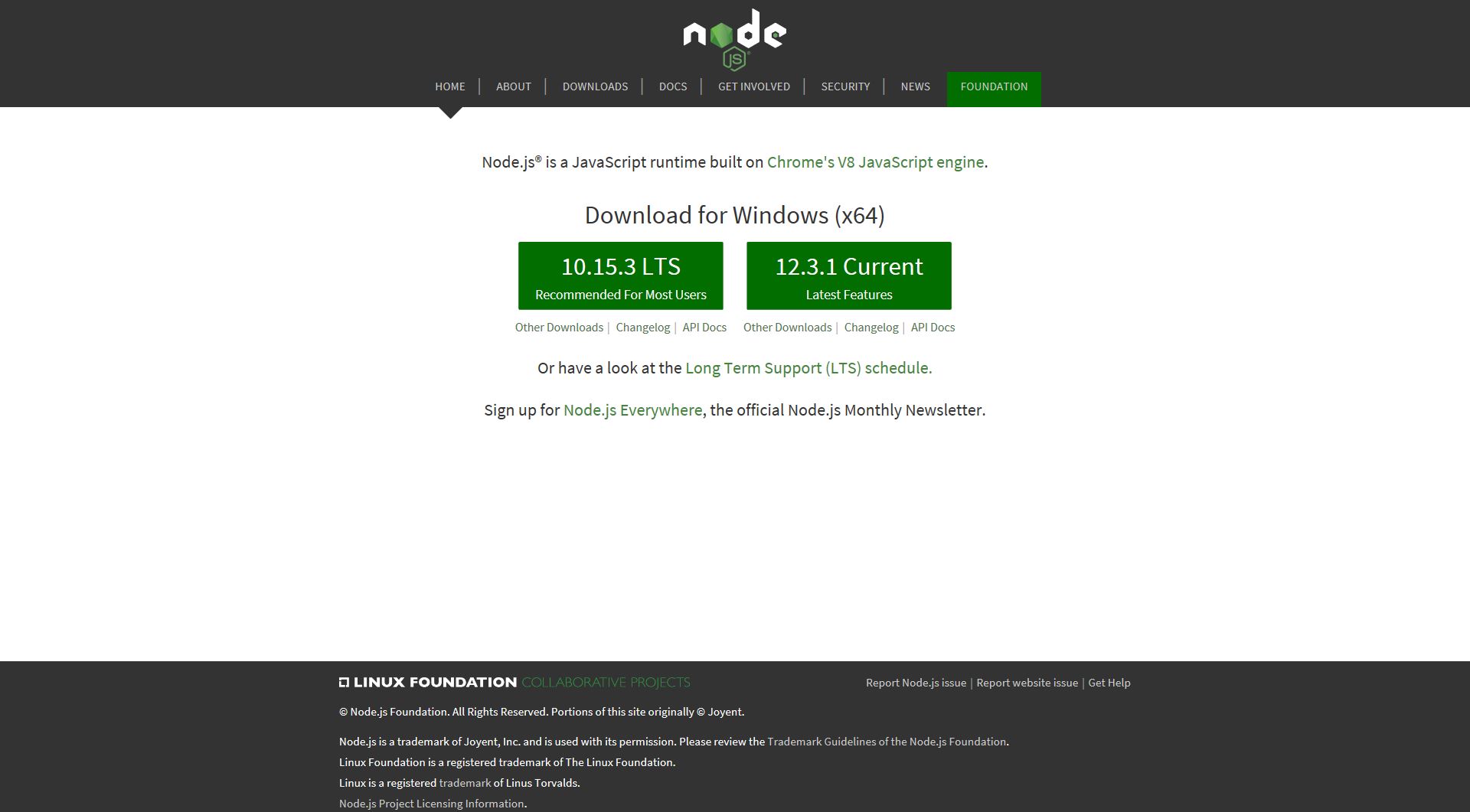
- Install latest nodejs and npm
- Clone the github repo
- Delete node_modules folder if exists
- Install dependencies by typing npm install
- Start ElectroLens by typing npm start
Example 1: visualize benzene electronic structure
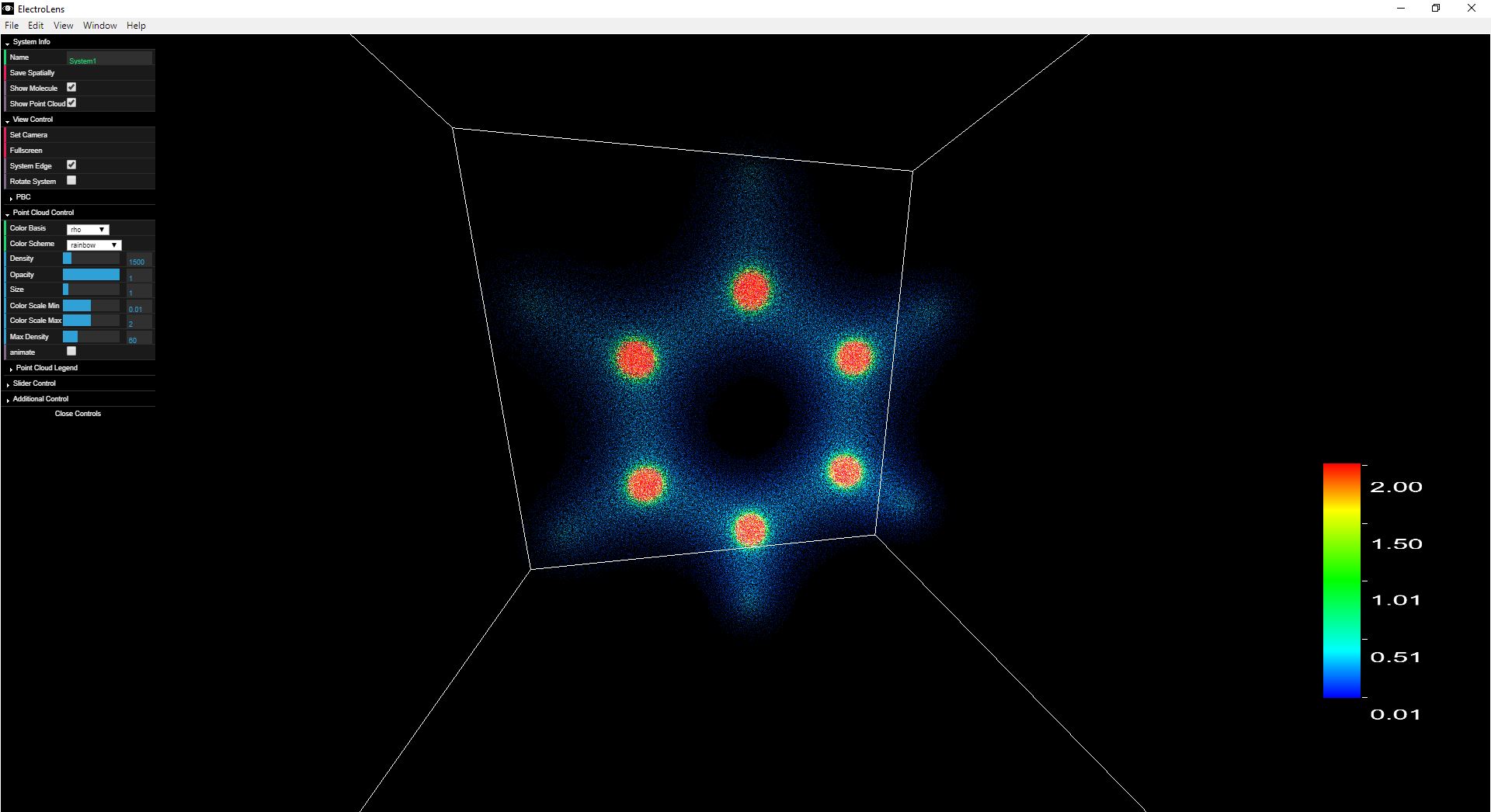
Benzene 3D View
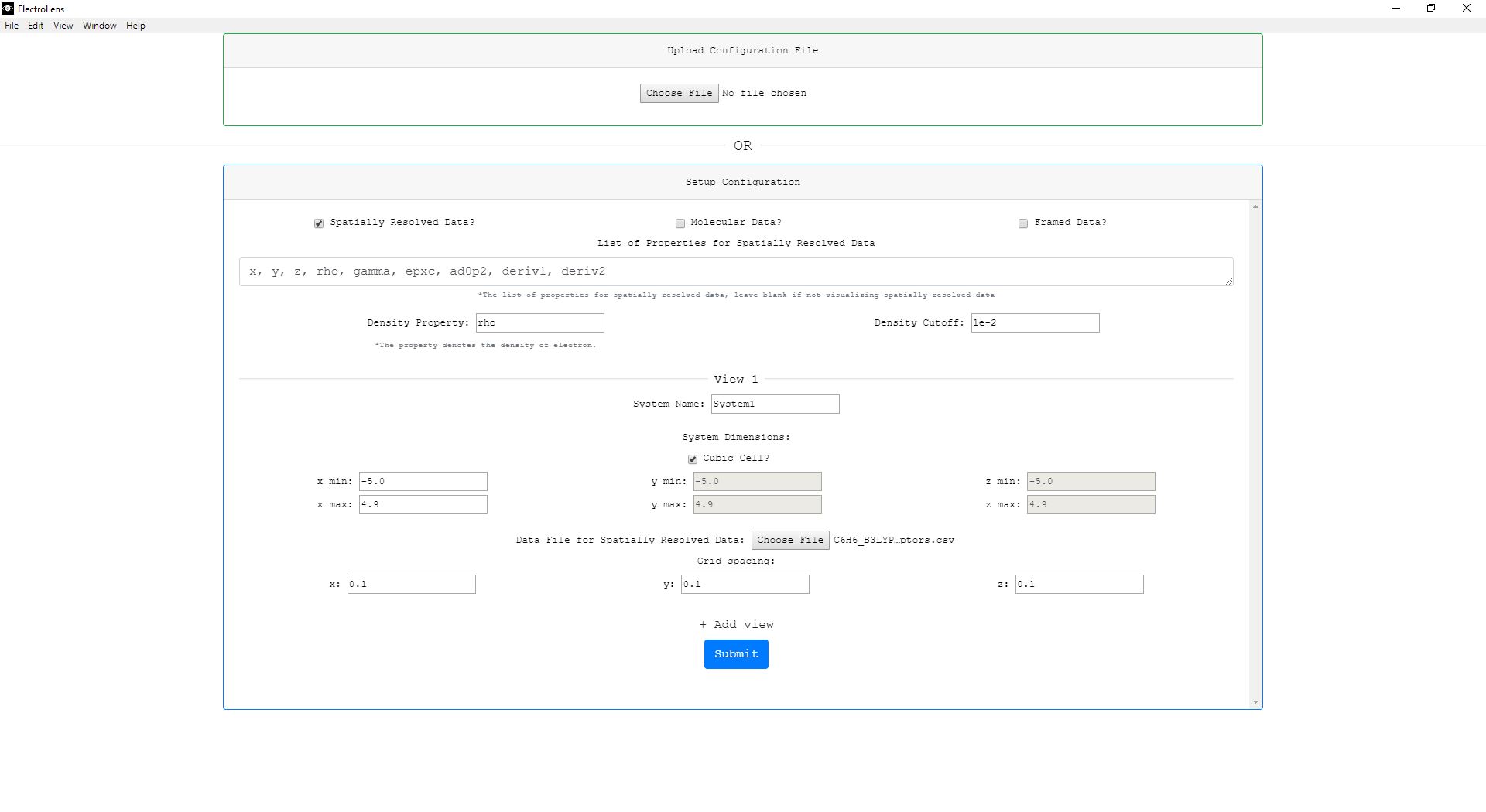
View Configuration
Loading the 3D view
- With predefined configuration file
- Go to "ElectroLens/Examples/example_configuration_files/"
- Open the "view_setp_example1.json" file with a text editor
- Go to line 8 ("dataFilename" for "spatiallyResolvedData") and change it to the full path of "/Examples/example_data/C6H6_electron_desnity_with_descriptors.csv"
- Start ElectroLens by typing npm start
- In
"Upload Configuration File" (green box), click"Choose File" and upload "view_setp_example1.json"
- Manually define configuration
- Start ElectroLens by typing npm start
- In Setup configuration (blue box) check Spatially Resolved Data?
- In the List of Properties for Spatially Resolved Data text area below, enter "x, y, z, rho, gamma, epxc, deriv1, deriv2" (no quotation mark)
- In View 1, upload the "CO2_electron_desnity_with_descriptors.csv" file in "ElectroLens/Examples/example/data"
- Leave the rest as default (as shown in the picture Above), and click Submit
- With predefined configuration file
View Customization
- Once you have the 3D view, you can customize it via the option box on the left
- PBC: add periodic replicates
- Point Cloud Control: customize point cloud view
- Color basis - property coded by color
- Color scheme - scheme for color code
- Density - density of the point cloud
- Size - size of each point
- Color scale min/max - adjust color scale
- Point cloud legend - adjust the legend
- Slider Control: set the spatial ranges of data to be visualized
Example 2: 2D Plots and Selection
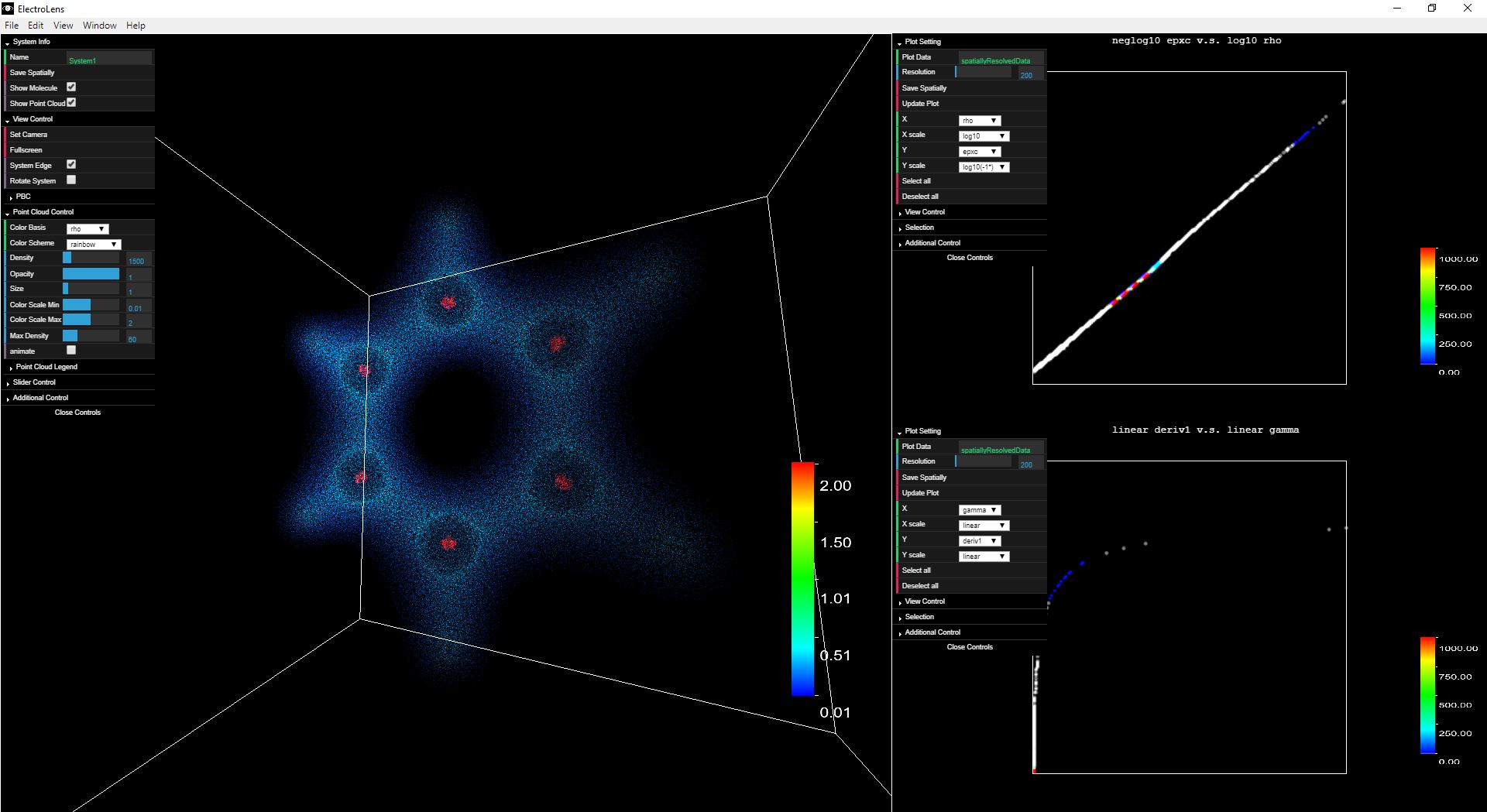
Benzene 2D plots and selection
Add 2D plots
- On the fly
- Start ElectroLens and load the 3D view as in Example 1
- Simply press a or + to add a 2D plot
- Adjust the X, Y axis properties and scales via the option box of the plot
- Remember to click Update Plot to reflect the changes
- Pre-defined configuration file
- Go to "ElectroLens/Examples/example_configuration_files/"
- Open the "view_setp_example2.json" file with a text editor
- Go to line 8 ("dataFilename" for "spatiallyResolvedData") and change it to the full path of that file (as in example 1)
- Go to line 14 - 17 to change the X, Y axis properties and X, Y axis scales respectively
- Start ElectroLens by typing npm start
- In
"Upload Configuration File" (green box), click"Choose File" and upload "view_setp_example2.json"
- On the fly
2D plots Customization
- Once you have the 2D plots, you can customize them via the option boxes of each plot
- Plot Setting
- Resolution - resolution of the heat map
- Update Plot - update the 2D plot. *** MUST CLICK to reflect any changes in "Plot Setting" ***
- X - X axis property
- X - X axis scale
- Y - Y axis property
- Y - Y axis scale
- Select All - select all data points
- Deselect All - deselect all data points
- View Control: change the color scheme and point sizes of the plot
Selection
To select points on the 2D plot and show the corresponding region in the 3D view- Deselect all datapoints, the 3D view should now be blank
- In the option box of 2D plot, go to Selection and check with plane (or press 1 for shortcut)
- Drag seletion box on the 2D plot to selection datapoints
- Try with the other option: Select with brush (press 2 for shortcut)
Example 3: visualize MD trajectory of 15 water
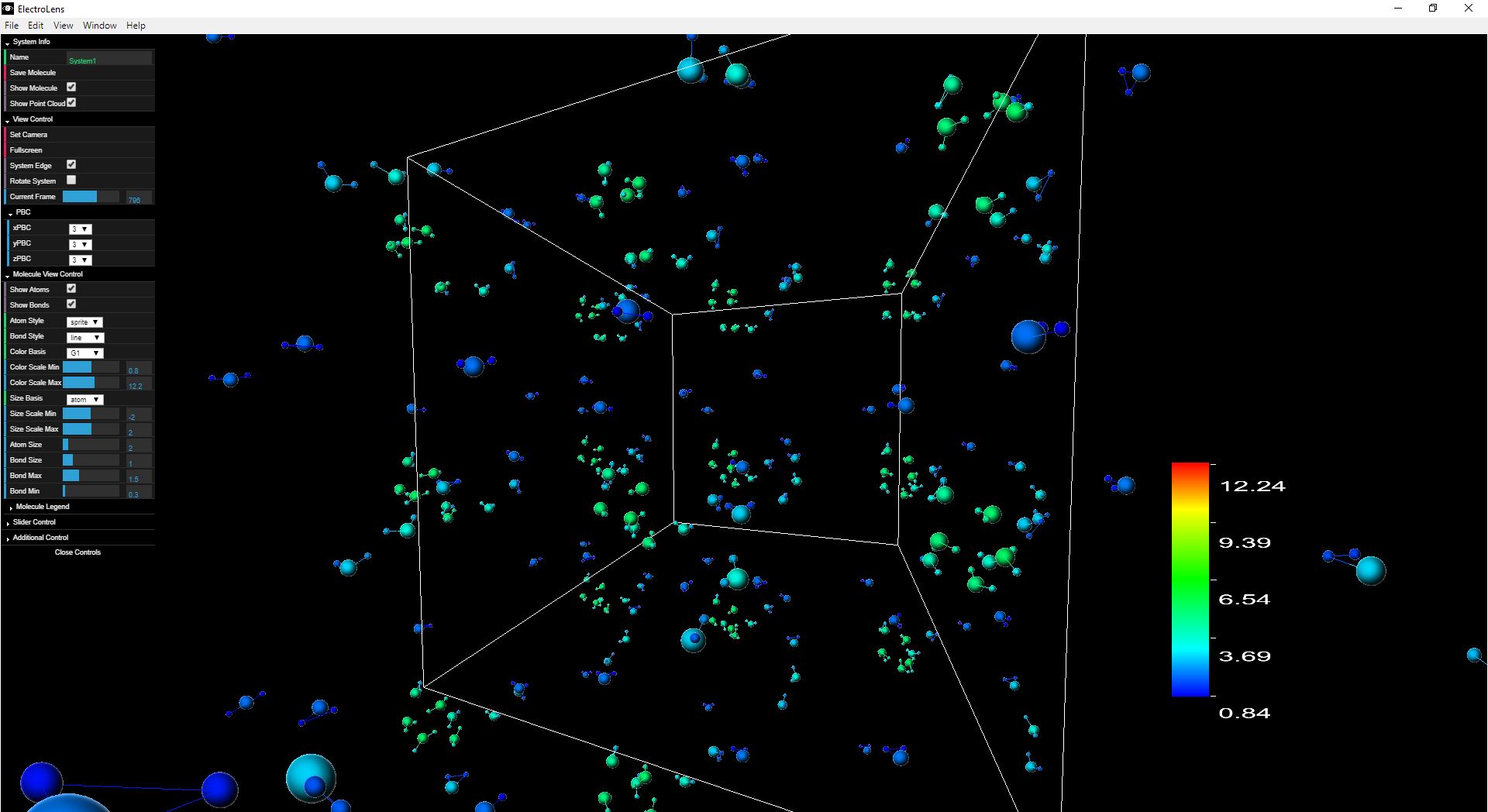
Water cluster 3D View
View Configuration
Loading the 3D view
- With predefined configuration file
- Go to "ElectroLens/Examples/example_configuration_files/"
- Open the "view_setp_example3.json" file with a text editor
- Go to line 7 ("dataFilename" for "moleculeData") and change it to the full path of that file
- Start ElectroLens by typing npm start
- In
"Upload Configuration File" (green box), click"Choose File" and upload "view_setp_example3.json"
- Manually define configuration
- Start ElectroLens by typing npm start
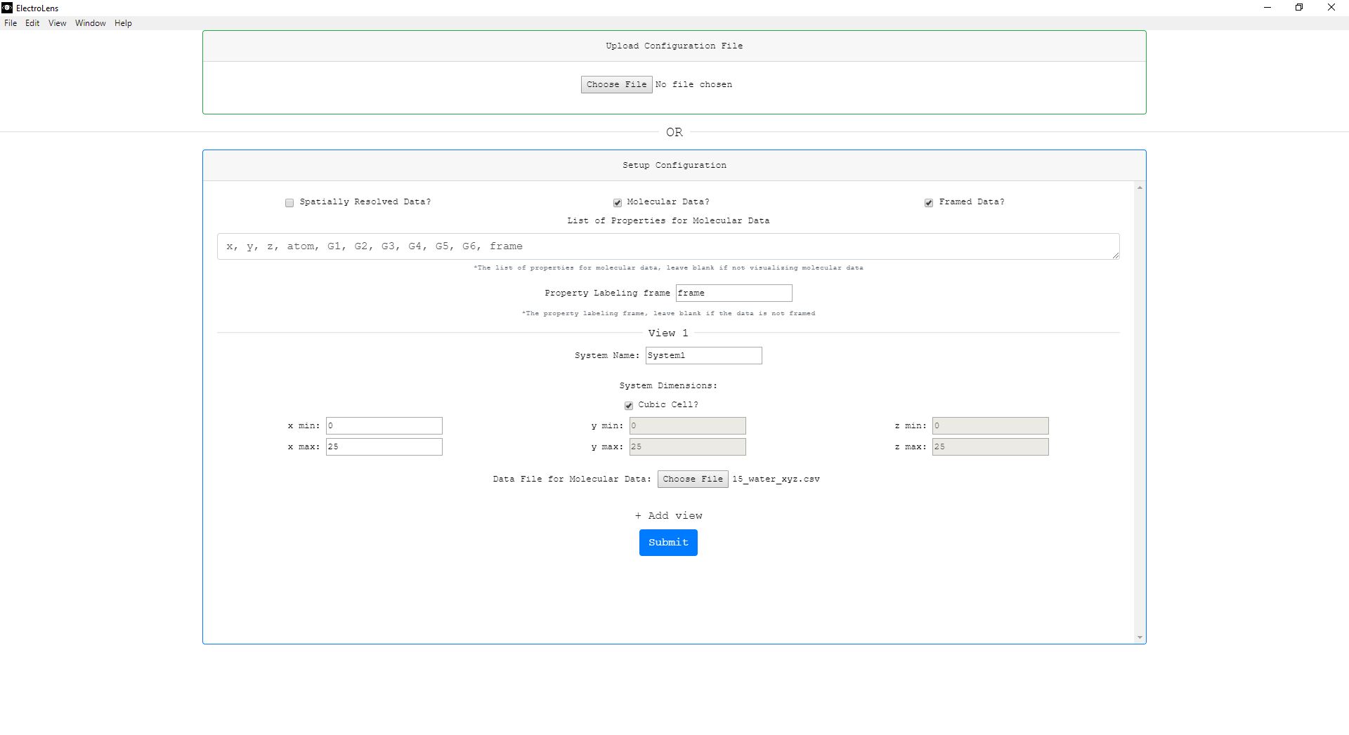
- In Setup configuration (blue box) check Molecular Data? and Framed Data?
- In the List of Properties for Molecular Data text area below, enter "x, y, z, atom, G1, G2, G3, G4, G5, G6, frame" (no quotation mark)
- In View 1, upload the 15_water_MD_with_Gaussian_fingerprints.csv file in "ElectroLens/Examples/example/data"
- Change the system dimemsion to be 0 for xmin, ymin, zmin and 25 for xmax, ymax, zmax
- Leave the rest as default (as shown in the picture Above), and click Submit
- With predefined configuration file
View Customization
- Once you have the 3D view, you can customize it via the option box on the left
- Drag the "Current Frame" bar in "View Control" to view different images in the trajectory
- PBC: add periodic replicates
- Molecule Control: customize point cloud view
- Atom style - style for drawing atoms (sprite is the much cheaper option)
- Bond style - style for drawing atoms (line is the much cheaper option)
- Color basis - property coded by color
- Color scale min/max - adjust color scale
- Size basis - property coded by atom size
- Size scale min/max - adjust color atom size
- Bond max/min - the max/min distance to draw bonds between 2 atoms
- Molecule legend - adjust the legend
Example 4: 2D Plots and Selection for Molecular Data
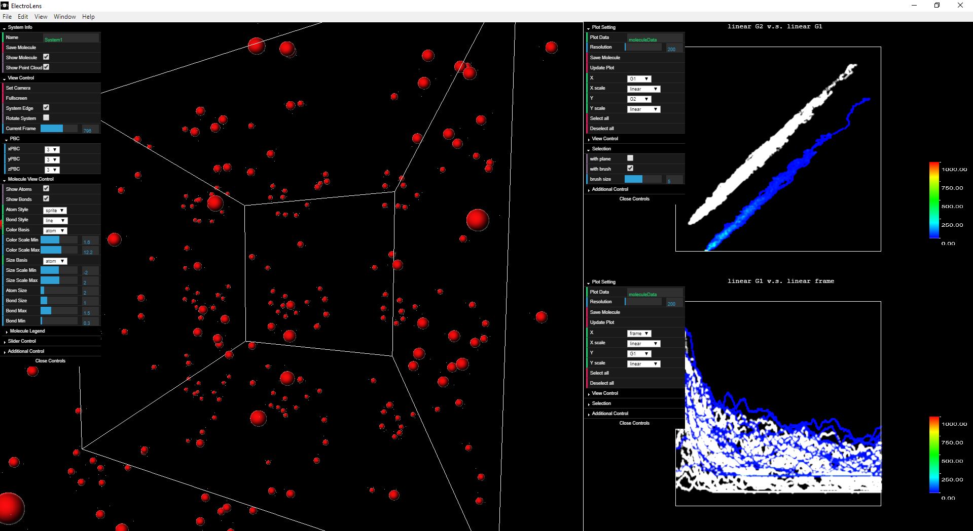
Water cluster 2D plots and selection
Add 2D plots
- On the fly
- Start ElectroLens and load the 3D view as in Example 3
- Simply press a or + to add a 2D plot
- Adjust the X, Y axis properties and scales via the option box of the plot
- Remember to click Update Plot to reflect the changes
- On the fly
2D plots Customization
- Once you have the 2D plots, you can customize them via the option boxes of each plot
- Plot Setting
- Resolution - resolution of the heat map
- Update Plot - update the 2D plot. *** MUST CLICK to reflect any changes in "Plot Setting" ***
- X - X axis property
- X - X axis scale
- Y - Y axis property
- Y - Y axis scale
- Select All - select all data points
- Deselect All - deselect all data points
- View Control: change the color scheme and point sizes of the plot
Selection
To select points on the 2D plot and show the corresponding region in the 3D view- Deselect all datapoints, the 3D view should now be blank
- In the option box of 2D plot, go to Selection and check with plane (or press 1 for shortcut)
- Drag seletion box on the 2D plot to selection datapoints
- Try with the other option: Select with brush (press 2 for shortcut)
Data Structure
ElectroLens uses csv (comma separated value) as the default file type for data
Depend on the type of descriptors (electronic structure or atomistic), slightly different properties are needed
To visualize framed data (trajectories for atoms or electronic structures), one extra property is needed
Electronic Structure Data
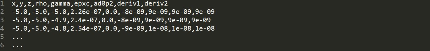 Data structure for electronic structure data
- Each row corresponds to a data point, and each column corresponds to a property
- Properties x, y, z and a property that corresponds to [density] (in this case "rho") are needed
Atomistic Data
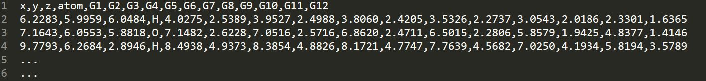 Data structure for atomistic data
- Each row corresponds to a data point, and each column corresponds to a property
- Properties x, y, z and atom (symbol for the corresponding element) are needed
Framed Data
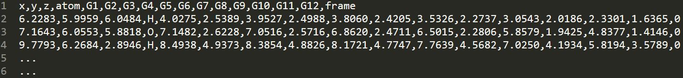 Data structure for framed data
- If the data to be visualized is framed (e.g. trajectory), simply add a column that corresponds to the [frame number] (in this case "frame")
- You can give it any name, just remember to specify it on the configuration form
- Works not only for atomistic trajectories, but also electronic structure trajectories